Analysis and Vizualization

The next step is to analyse the results created by OpenDC. When running a simulation, OpenDC generates five types of output files. The output folder has the following structure:

[1]    output 📁
[2]    ├── simple 📁
[3]    │   ├── raw-output 📁
[4]    │   │   |── 0 📁
[5]    │   │   |   └── seed=0 📁
[6]    |   |   |       └── host.parquet 📄
[7]    |   |   |       └── powerSource.parquet 📄
[8]    |   |   |       └── service.parquet 📄
[9]    |   |   |       └── task.parquet 📄
[10]   │   │   |── 1 📁
[11]   │   │   |   └── seed=0 📁
[12]   |   |   |       └── host.parquet 📄
[13]   |   |   |       └── powerSource.parquet 📄
[14]   |   |   |       └── service.parquet 📄
[15]   |   |   |       └── task.parquet 📄
[16]   |   ├── simulation-analysis 📁
[17]   |   └── trackr.json 📄

The output of an experiment is put inside the output folder, in a folder with the given experiment name. The output of the experiment executed in the previous part of this tutorial can be found in the folder named "simple"[2].

The output folder of an experiment consist of one file and two folders:

raw-output contains all raw output files generated during the simulation
simulation-analysis contains automatic analysis done by OpenDC Note: this is only relevant when using M3SA and can be ignored in this tutorial
trackr.json contains the parameters used in the simulations executed during the experiment. This file can be very helpful when running a large number of experiments

5. raw-output

The raw-output folder is subdivided into multiple folders, each representing a single simulation run by OpenDC. As we explained in the first part of the tutorial, users can provide multiple value for certain parameters. Consequently, OpenDC will run a simulation for each combination of parameters.

In this tutorial, we have run two simulations resulting in two folders. The trackr file can be used to determine which output is related to which configuration. Each simulation is divided into multiple folders depending on how many times the simulation is run. Using the runs parameter in the experiment files, a user can execute the same simulation multiple times. Each run is executed using a different random seed. This can be usefull when a simulation uses random models.

During a simulation, multiple parquet files are created with information regarding different aspects. We advise users to use the Pandas library for reading the output files. This will make analysis and vizualization easy.

Input

import pandas as pd
import numpy as np
import matplotlib.pyplot as plt

df_host_small = pd.read_parquet("output/simple/raw-output/0/seed=0/host.parquet")
df_powerSource_small = pd.read_parquet("output/simple/raw-output/0/seed=0/powerSource.parquet")
df_task_small = pd.read_parquet("output/simple/raw-output/0/seed=0/task.parquet")
df_service_small = pd.read_parquet("output/simple/raw-output/0/seed=0/service.parquet")

df_host_big = pd.read_parquet("output/simple/raw-output/1/seed=0/host.parquet")
df_powerSource_big = pd.read_parquet("output/simple/raw-output/1/seed=0/powerSource.parquet")
df_task_big = pd.read_parquet("output/simple/raw-output/1/seed=0/task.parquet")
df_service_big = pd.read_parquet("output/simple/raw-output/1/seed=0/service.parquet")

print(f"The small dataset has {len(df_service_small)} service samples.")
print(f"The big dataset has {len(df_service_big)} service samples.")

Output

The small dataset has 12026 service samples. The big dataset has 1440 service samples.

Host

The host file contains all metrics regarding the hosts.

Examples of how to use this information:

How much power is each host drawing?
What is the average utilization of hosts?

Input

print(f"The host file contains the following columns:\n {np.array(df_host_small.columns)}\n")
print(f"The host file consist of {len(df_host_small)} samples\n")
df_host_small.head()

Output

The host file contains the following columns: ['timestamp' 'timestamp_absolute' 'host_name' 'cluster_name' 'core_count' 'mem_capacity' 'tasks_terminated' 'tasks_running' 'tasks_error' 'tasks_invalid' 'cpu_capacity' 'cpu_usage' 'cpu_demand' 'cpu_utilization' 'cpu_time_active' 'cpu_time_idle' 'cpu_time_steal' 'cpu_time_lost' 'power_draw' 'energy_usage' 'embodied_carbon' 'uptime' 'downtime' 'boot_time']

The host file consist of 12026 samples

	timestamp	timestamp_absolute	host_name	cluster_name	core_count	mem_capacity	tasks_running	...	cpu_time_active	cpu_time_idle	power_draw	energy_usage	embodied_carbon	uptime	boot_time
0	3600000	1376318146000	H01	C01	12	140457600000	8	...	20173	3579827	201.169	724034	22.8311	3600000	1376314546000
1	7200000	1376321746000	H01	C01	12	140457600000	8	...	20804	3579196	201.326	724161	22.8311	3600000	1376314546000
2	10800000	1376325346000	H01	C01	12	140457600000	8	...	20156	3579844	201.158	724031	22.8311	3600000	1376314546000
3	14400000	1376328946000	H01	C01	12	140457600000	8	...	20457	3579543	201.376	724091	22.8311	3600000	1376314546000
4	18000000	1376332546000	H01	C01	12	140457600000	8	...	20021	3579979	201.159	724004	22.8311	3600000	1376314546000

Tasks

The host file contains all metrics regarding the executed tasks.

Examples of how to use this information:

When is a specific task executed?
How long did it take to finish a task?
On which host was a task executed?

Input

print(f"The task file contains the following columns:\n {np.array(df_task_small.columns)}\n")
print(f"The task file consist of {len(df_task_small)} samples\n")
df_task_small.head()

Output

The task file contains the following columns: ['timestamp' 'timestamp_absolute' 'task_id' 'task_name' 'host_name' 'mem_capacity' 'cpu_count' 'cpu_limit' 'cpu_usage' 'cpu_demand' 'cpu_time_active' 'cpu_time_idle' 'cpu_time_steal' 'cpu_time_lost' 'uptime' 'downtime' 'num_failures' 'num_pauses' 'schedule_time' 'submission_time' 'finish_time' 'task_state']

The task file consist of 343430 samples

	timestamp	timestamp_absolute	task_id	task_name	host_name	mem_capacity	cpu_count	cpu_usage	cpu_demand	...	uptime	schedule_time	finish_time	task_state
0	3600000	1376318146000	00000000-0000-0000-5449-6ad67bd2634c	205		20972	8	0	0	...	0	nan	nan	PROVISIONING
1	3600000	1376318146000	00000000-0000-0000-f88b-b8a8724c81ec	1023	H01	260	1	11.704	11.704	...	3600000	0	nan	RUNNING
2	3600000	1376318146000	00000000-0000-0000-6963-0f7593d108c3	378		8360	2	0	0	...	0	nan	nan	PROVISIONING
3	3600000	1376318146000	00000000-0000-0000-12c0-15a97019e937	466		3142	4	0	0	...	0	nan	nan	PROVISIONING
4	3600000	1376318146000	00000000-0000-0000-451e-521296a7eea1	915		262	1	0	0	...	0	nan	nan	PROVISIONING

PowerSource

The task file contains all information about the power sources. Examples of use cases:

What is the total energy used during the workload?

Input

print(f"The task file contains the following columns:\n {np.array(df_powerSource_small.columns)}\n")
print(f"The power file consist of {len(df_powerSource_small)} samples\n")
df_powerSource_small.head()

Output

The task file contains the following columns: ['timestamp' 'timestamp_absolute' 'source_name' 'cluster_name' 'power_draw' 'energy_usage' 'carbon_intensity' 'carbon_emission']

The power file consist of 12026 samples

	timestamp	timestamp_absolute	source_name	cluster_name	power_draw	energy_usage
0	3600000	1376318146000	PowerSource	C01	201.169	724034
1	7200000	1376321746000	PowerSource	C01	201.326	724161
2	10800000	1376325346000	PowerSource	C01	201.158	724031
3	14400000	1376328946000	PowerSource	C01	201.376	724091
4	18000000	1376332546000	PowerSource	C01	201.159	724004

Service

The service file contains genaral information about the experiments.

Example use cases of this file:

How many tasks are running?
How many hosts are active?

Input

print(f"The service file contains the following columns:\n {np.array(df_service_small.columns)}\n")
print(f"The service file consist of {len(df_service_small)} samples\n")
df_service_small.head()

Output

The service file contains the following columns: ['timestamp' 'timestamp_absolute' 'hosts_up' 'hosts_down' 'tasks_total' 'tasks_pending' 'tasks_active' 'tasks_completed' 'tasks_terminated']

The service file consist of 12026 samples

	timestamp	timestamp_absolute	hosts_up	tasks_total	tasks_pending	tasks_active
0	3600000	1376318146000	1	44	36	8
1	7200000	1376321746000	1	44	36	8
2	10800000	1376325346000	1	44	36	8
3	14400000	1376328946000	1	44	36	8
4	18000000	1376332546000	1	44	36	8

6. Aggregating Ouput

To get a better understanding of the experiment output, we would like to aggregate them into single values. This will also allow us to determine the differences between the two datacenter sizes.

We want to compare the two simulations in the following three aspects:

runtime
average utilization
energy usage

Runtime

Input

# Getting the end time of the simulation, and thus the runtime
runtime_small = df_service_small["timestamp"].max()
runtime_big = df_service_big["timestamp"].max()

# Converting the runtime from ms to timedelta
runtime_small_td = pd.to_timedelta(runtime_small, unit='ms')
runtime_big_td = pd.to_timedelta(runtime_big, unit='ms')

# Printing the results 
print(f"The runtime of the small datacenter is {runtime_small_td} hours")
print(f"The runtime of the big datacenter is {runtime_big_td} hours")

Output

The runtime of the small dataset is 501 days 01:53:08 hours The runtime of the big dataset is 59 days 23:44:48 hours

Using a larger datacenter allows for paralel execution of tasks, and thus a much smaller runtime.

Power Draw

Input

# Getting the end time of the simulation, and thus the runtime
runtime_small = df_host_small["cpu_utilization"].mean()
runtime_big = df_host_big["cpu_utilization"].mean()

# Convert utlization to percentage
runtime_small = runtime_small * 100
runtime_big = runtime_big * 100

# Printing the results
print(f"The average CPU utilization of the small datacenter is {runtime_small:.2f} %")
print(f"The average CPU utilization of the big datacenter is {runtime_big:.2f} %")

Output

The average CPU utilization of the small datacenter is 11.84 % The average CPU utilization of the big datacenter is 10.96 %

As expected, the average utilization of the big datacenter is lower than that of the smaller datacenter.

Energy Usage

Input

# Get the total energy usage during the simulation
energy_small = df_powerSource_small["energy_usage"].sum()
energy_big = df_powerSource_big["energy_usage"].sum()

# Convert energy to kWh
energy_small = energy_small / 3_600_000
energy_big = energy_big / 3_600_000

# Printing the results
print(f"The total energy usage of the small datacenter is {energy_small:.2f} kWh")
print(f"The total energy usage of the big datacenter is {energy_big:.2f} kWh")

Output

The total energy usage of the small datacenter is 2690.83 kWh The total energy usage of the big datacenter is 2876.43 kWh

Surprisingly, the big data center uses more energy than the small datacenter, eventhough its runtime is almost 10 times smaller. This is caused by the high number of hosts still drawing power, even when idle.

7. Vizualization

To getting even more insight into the results, we can plot the results.

Active tasks

First we plot the number of active tasks during the workload

Input

plt.plot(df_service_small["timestamp"]/3_600_000 / 24, df_service_small["tasks_active"], label="Small datacenter")
plt.plot(df_service_big["timestamp"]/3_600_000 / 24, df_service_big["tasks_active"], label="Big datacenter")
plt.xlabel("Time [days]")
plt.ylabel("Number of active tasks")
plt.title("Number of active tasks over time")
plt.legend()

Output

<matplotlib.legend.Legend at 0x785d21c5b410>

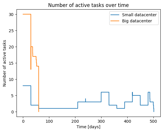
Because of its size, the big datacenter is able to run up to 30 tasks in parallel. In contrast, the small datacenter cannot run more than 8 tasks.

Energy Usage

Below we show the energy usage over time for the two data centers.

Input

# Sum the energy usage of each power source at each timestamp
energy_usage_big = df_powerSource_big.groupby("timestamp")["energy_usage"].sum()

# Compute a windowed (rolling) average of energy usage with a window size of 50 samples
window_size = 100
energy_usage_small_rolling = df_powerSource_small["energy_usage"].rolling(window=window_size, min_periods=1).mean()
energy_usage_big_rolling = energy_usage_big.rolling(window=window_size, min_periods=1).mean()

plt.plot(df_powerSource_small["timestamp"] / 3_600_000 / 24, energy_usage_small_rolling / 3_600_000, label="Small datacenter")
plt.plot(energy_usage_big_rolling.index / 3_600_000 / 24, energy_usage_big_rolling / 3_600_000, label="Big datacenter")
plt.xlabel("Time [days]")
plt.ylabel("Energy usage [kWh]")
plt.title("Energy usage of the datacenters")
plt.ylim([0, None])
plt.legend()

Output

<matplotlib.legend.Legend at 0x785d3829cef0>

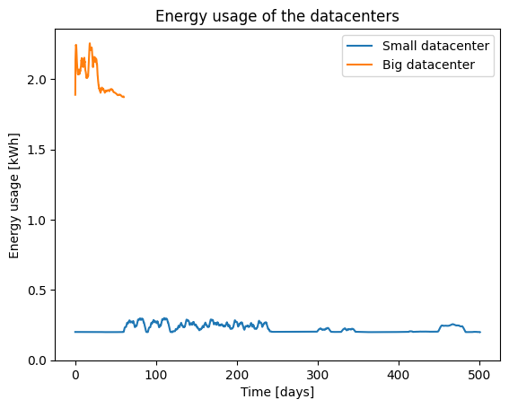
Because of its size, the big datacenter is using a lot more energy compared to the small datacenter.

Analysis and Vizualization

5. raw-output​

Input​

Output​

Host​

Input​

Output​

Tasks​

Input​

Output​

PowerSource​

Input​

Output​

Service​

Input​

Output​

6. Aggregating Ouput​

Runtime​

Input​

Output​

Power Draw​

Input​

Output​

Energy Usage​

Input​

Output​

7. Vizualization​

Active tasks​

Input​

Output​

Energy Usage​

Input​

Output​

5. raw-output

Input

Output

Host

Input

Output

Tasks

Input

Output

PowerSource

Input

Output

Service

Input

Output

6. Aggregating Ouput

Runtime

Input

Output

Power Draw

Input

Output

Energy Usage

Input

Output

7. Vizualization

Active tasks

Input

Output

Energy Usage

Input

Output